> For the complete documentation index, see [llms.txt](https://navixy.com/docs/llms.txt). Markdown versions of documentation pages are available by appending `.md` to page URLs; this page is available as [Markdown](https://navixy.com/docs/user/guide/account/iot-logic/flow-management/flow-configuration-example.md).
# Flow configuration example
A step-by-step example showing how to build an IoT Logic flow that collects device telemetry, calculates derived metrics, and forwards enriched data externally.
This example demonstrates how to configure a flow that collects data from IoT devices, performs calculations to derive business-relevant metrics, and forwards the enriched data to an external system. The example uses a linear flow pattern that can be adapted to various industry use cases.
## Business scenario
In this scenario, an organization has deployed GPS devices on their assets and needs to process data from these devices for business analytics. The organization receives the following parameters directly from their tracking devices:
* `speed`: Vehicle speed in kilometers per hour
* `temperature`: Environmental temperature in Celsius
* `odometer`: Distance traveled in kilometers
* `ignition`: Engine ignition status (1 = on, 0 = off)
* `fuel_level`: Current fuel level measurement
* `pressure_psi`: Pressure reading in PSI
* `voltage`: Battery voltage in volts
* `throttle`: Throttle pedal position from CAN bus (0-255)
* `fuel_level_1`: First fuel tank level measurement
* `fuel_level_2`: Second fuel tank level measurement
The organization needs to:
1. Collect raw telemetry data from devices to maintain a complete record of asset operations
2. Convert measurement units to match their standard reporting format (imperial units) for consistency with existing business systems
3. Calculate time-based metrics that indicate usage patterns to optimize asset utilization and maintenance schedules
4. Create derived metrics to generate operational insights not directly provided by the hardware
5. Forward the enriched data to an external analysis system for integration with business intelligence platforms
6. Send unchanged raw data to Navixy for monitoring
This flow transforms the raw device data into a format that directly supports business decision-making while maintaining the integrity of the original measurements.
## Flow configuration steps
Follow these steps to build a comprehensive data transformation and forwarding flow:
{% stepper %}
{% step %}
### Create a new flow
Open IoT Logic. On the start page, click **Create Flow**. Enter *Asset Telemetry Processing* as the flow name, add a description (*"Collects device data, calculates derived metrics, and forwards to analytics platform."*), and ensure the **Flow enabled** toggle is switched on. Click **Confirm** to open the canvas.
{% endstep %}
{% step %}
### Configure the data source
1. Drag a **Data Source** node from the left menu to the workspace
2. Double-click on the node to open its configuration panel
3. In **Node name** type *Asset Trackers*
4. Select the devices to include in this flow from the filtered list
* For this example, select at least two devices with similar capabilities
5. Click **Apply** to save node configuration
{% endstep %}
{% step %}
### Set up basic data transformations
1. Drag an **Initiate Attribute** node from the left menu to the workspace
2. Connect the **Data Source** node to this **Initiate Attribute** node
3. Double-click the node to open its configuration
4. In **Node name** type *Unit conversions*
5. Create the following attributes for unit conversion (all examples use short syntax, referring to the latest attribute values without validity check):
1. Add a new attribute for speed conversion (km/h to mph): 1. Attribute name: *speed\_mph* 2. Value: `speed/1.609`
2. Add a new attribute for temperature conversion (Celsius to Fahrenheit): 1. Attribute name: *temperature\_F* 2. Value: `temperature*1.8 + 32`
3. Add a new attribute for distance conversion (kilometers to miles): 1. Attribute name: *distance\_miles* 2. Value: `odometer/1.609`
4. Add a new attribute for pressure conversion (PSI to Bar): 1. Attribute name: *pressure\_bar* 2. Value: `pressure_psi * 0.06895`
6. Click **Apply** to save node configuration
{% hint style="info" %}
For explanations on calculations introduced in this step, see [Basic unit conversions](#basic-unit-conversions)
{% endhint %}
{% endstep %}
{% step %}
### Create advanced calculated metrics
1. Drag another **Initiate Attribute** node from the left menu to the workspace
2. Connect the first **Initiate Attribute** node to this new one
3. Double-click on the node to open its configuration
4. In **Node name** type *Advanced calculations*
5. Create the following attributes for advanced metrics:
1. Add an attribute for temperature change detection:
1. Attribute name: *temperature\_change*
2. Value: `value('temperature', 0, 'valid') - value('temperature', 1, 'valid')`
3. `genTime('temperature', 0, 'valid')`
2. Add an attribute for finding time elapsed between two last readings:
1. Attribute name: *time\_between\_readings\_ms*
2. Value: `srvTime('speed', 0, 'valid') - srvTime('speed', 1, 'valid')`
3. Generation time: `genTime('speed', 0, 'valid')`
3. Add an attribute for round temperature to nearest integer:
1. Attribute name: *temperature\_rounded*
2. Value: `math:round(value('temperature', 0, 'valid'))`
4. Add an attribute for standardized value calculation (normalizing fuel level to 0-100%):
1. Attribute name: *fuel\_level\_percent*
2. Value: `(value('fuel_level', 0, 'valid') - 0) / (100 - 0) * 100`
5. Add an attribute for battery charge percentage calculation:
1. Attribute name: *battery\_percentage*
2. Value: `(value('voltage', 0, 'valid') - 11) / (14 - 11) * 100`
6. Add an attribute for throttle position calculation:
1. Attribute name: *throttle\_percentage*
2. Value: `value('throttle', 0, 'valid') / 255 * 100`
7. Add an attribute for average fuel level from multiple sensors:
1. Attribute name: *avg\_fuel\_level*
2. Value: `(value('fuel_level_1', 0, 'valid') + value('fuel_level_2', 0, 'valid')) / 2`
6. Click **Apply** to save node configuration
{% hint style="info" %}
For explanations on calculations introduced in this step, see [Advanced metrics calculations](#advanced-metrics-calculations).
{% endhint %}
{% endstep %}
{% step %}
### Configure the output endpoint
1. Drag an **Output Endpoint** node from the left menu to the workspace
2. Connect the second **Initiate Attribute** node to this **Output Endpoint** node
3. Click on the node to open its configuration
4. Configure the following settings:
1. **Endpoint type**: *MQTT endpoint*
2. **Endpoint name**: *Analytics Platform*
3. **Protocol**: default *Navixy Generic Protocol (JSON)*
4. **IP/Domain**: Enter the destination system address (e.g., "*analytics.example.com*")
5. **Port**: *8883* (default for MQTT, you can leave it empty)
6. **Enable SSL**: *toggle on*
7. **MQTT Version**: *5.0*
8. **MQTT Client ID**: *asset-telemetry-client*
9. **Topic**: *telemetry/assets/raw*
10. **QoS**: *1*
11. **MQTT Authentication**: *Yes* (if required by your destination system)
12. **MQTT Login and Password**: Enter credentials if applicable
5. Click **Create** to save node configuration
{% endstep %}
{% step %}
### Add Default Output endpoint
1. Drag an **Output Endpoint** node from the left menu to the workspace
2. In **Mode** select **Default endpoint**
3. Click **Save** to apply node configuration
4. Connect the *Asset Trackers* (**Data Source**) node to it
This ensures that the raw data is sent to Navixy directly from the devices, without any transformations and enrichments.
{% endstep %}
{% step %}
### Save and test the flow
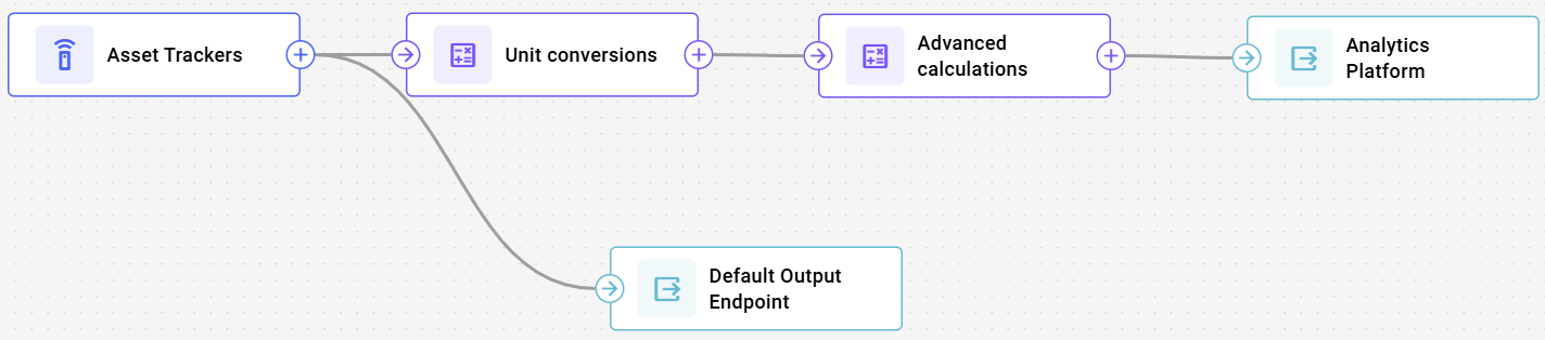
Your final configuration will look like this:
Click the **Save flow** button on the **Nodes** pane to store your flow configuration.
{% endstep %}
{% endstepper %}
{% hint style="success" %}
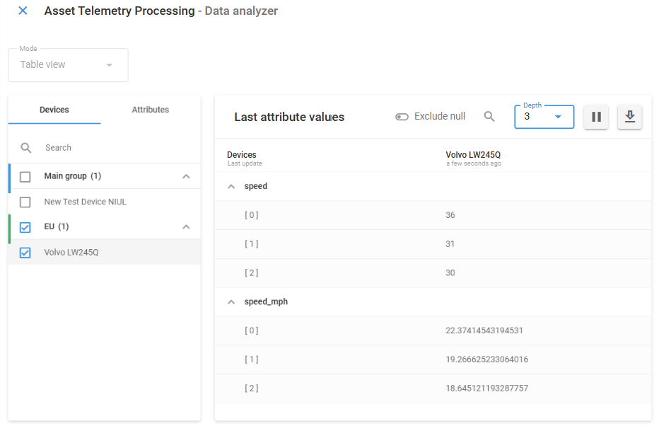
Use [Data Stream Analyzer (DSA)](/docs/user/guide/account/iot-logic/data-stream-analyzer.md) to monitor incoming data to verify:
* Devices are sending data to the flow
* Calculations are working as expected
* Data is being forwarded to the destination For example, let’s check that speed conversions are calulated correctly on a truck. To do it in DSA, select the **Volvo** device and attributes **speed** and **speed\_mph**:\
All good! Data is received and converted successfully.
{% endhint %}
## Data transformations explained
Let's examine the key calculations used in this flow.
### Basic unit conversions
The first **Initiate attribute node** performs straightforward unit conversions:
* **Speed**: Converts km/h to mph by dividing by 1.609
* **Temperature**: Converts Celsius to Fahrenheit using the formula °F = °C × 1.8 + 32
* **Distance**: Converts kilometers to miles by dividing by 1.609
* **Pressure**: Converts PSI to Bar by multiplying by 0.06895, making it compatible with international pressure measurement standards
These conversions ensure consistency with standard reporting formats and make the data immediately usable for analysis. Unit conversions are particularly valuable for multinational organizations that operate across regions with different measurement standards.
### Advanced metrics calculations
The second **Initiate attribute node** performs more complex calculations:
* **Temperature change detection**: Calculates the difference between current and previous temperature readings to identify sudden changes. This helps detect equipment issues such as refrigeration failures in transport vehicles or HVAC problems in facilities. For example, a sudden 5°C rise in a refrigerated container might indicate a cooling system failure requiring immediate attention.
* **Generation time**: Using `genTime('temperature', 0, 'valid')` is crucial here because it preserves the exact timestamp when the temperature reading was generated by the device, ensuring accurate time-based analysis of temperature changes.
* **Server time**: The default value `now()` automatically captures when the server received the data. This timestamp doesn't need modifying, so leave this field empty during configuration.
* **Time between readings**: Measures the interval between consecutive data transmissions by comparing server timestamps. This calculation helps identify communication issues or validate that devices are reporting at expected frequencies. Irregular intervals might indicate connectivity problems, while consistent delays could suggest network congestion or device configuration issues.
* **Rounding values**: Applies mathematical rounding to temperature readings, reducing decimal precision to integers. This simplifies data visualization and reporting while reducing storage requirements for historical data. Rounded values are especially useful for dashboard displays and threshold-based alerts where decimal precision isn't necessary.
* **Generation time**: Specifying `genTime('speed', 0, 'valid')` connects this metadata directly to the original reading's timestamp, making it possible to analyze both the time interval and when it occurred.
* **Server time**: The default value `now()` automatically captures when the server received the data. This timestamp doesn't need modifying, so leave this field empty during configuration.
* **Standardized value calculation**: Normalizes raw sensor readings to a percentage scale (0-100%). This standardization makes it easier to compare readings across different sensor types and vehicle models. For fleet management, this allows consistent fuel level reporting regardless of the specific fuel sensor implementation in each vehicle model, enabling uniform low-fuel alerts and consumption analysis.
* **Battery charge percentage calculation**: Normalizes battery voltage readings (11V-14V range) to a 0-100% scale for easier monitoring. For example, a reading of 12.5V would be normalized to 50%, providing an intuitive indicator of battery health across different vehicle types.
* **Throttle position calculation**: Converts raw throttle position data (0-255 range) from the vehicle's CAN bus to a percentage scale. This standardization helps operators quickly understand driver behavior and vehicle performance without needing to interpret raw sensor values.
* **Average fuel level from multiple sensors**: Combines readings from two separate fuel sensors to produce a more accurate overall fuel level measurement. This is particularly valuable for vehicles with complex tank shapes or multiple tanks, where a single sensor might not provide reliable readings due to fuel shifting during movement.
## Example flow summary
This flow configuration demonstrates several key IoT Logic capabilities:
1. **Standardization**: Converts device-specific readings into standardized business metrics
2. **Enrichment**: Creates new, meaningful metrics not directly available from device sensors
3. **Transformation**: Changes units to match business reporting requirements
4. **Historical context**: Uses previous readings to calculate trend-based metrics
5. **Status determination**: Creates categorical values based on multiple sensor inputs
This combination of capabilities transforms raw device data into actionable business intelligence, directly supporting operational decision-making while maintaining the integrity of the original measurements.
---
# Agent Instructions
This documentation is published with GitBook. GitBook is the documentation platform designed so that both humans and AI agents can read, navigate, and reason over technical content effectively. Learn more at gitbook.com.
## Querying This Documentation
If you need additional information that is not directly available in this page, you can query the documentation by asking a question.
Perform an HTTP GET request on the following URL with the `ask` and `goal` query parameters:
```
GET https://navixy.com/docs/user/guide/account/iot-logic/flow-management/flow-configuration-example.md?ask=&goal=
```
`ask` is the immediate question: it should be specific, self-contained, and written in natural language.
`goal` is what the user is ultimately trying to achieve, the reason they need the answer. Sharing it helps GitBook give you a better, more relevant answer. A goal is most helpful when it describes the outcome the user wants rather than restating the question. For example, with `ask=how do I create an API token`, a goal like `automate deployments from our CI pipeline` lets GitBook tailor the answer to that use case.
The response will contain a direct answer to the question and relevant excerpts and sources from the documentation.
Use this mechanism when the answer is not explicitly present in the current page, you need clarification or additional context, or you want to retrieve related documentation sections.
 All good! Data is received and converted successfully.
{% endhint %}
## Data transformations explained
Let's examine the key calculations used in this flow.
### Basic unit conversions
The first **Initiate attribute node** performs straightforward unit conversions:
* **Speed**: Converts km/h to mph by dividing by 1.609
* **Temperature**: Converts Celsius to Fahrenheit using the formula °F = °C × 1.8 + 32
* **Distance**: Converts kilometers to miles by dividing by 1.609
* **Pressure**: Converts PSI to Bar by multiplying by 0.06895, making it compatible with international pressure measurement standards
These conversions ensure consistency with standard reporting formats and make the data immediately usable for analysis. Unit conversions are particularly valuable for multinational organizations that operate across regions with different measurement standards.
### Advanced metrics calculations
The second **Initiate attribute node** performs more complex calculations:
* **Temperature change detection**: Calculates the difference between current and previous temperature readings to identify sudden changes. This helps detect equipment issues such as refrigeration failures in transport vehicles or HVAC problems in facilities. For example, a sudden 5°C rise in a refrigerated container might indicate a cooling system failure requiring immediate attention.
* **Generation time**: Using `genTime('temperature', 0, 'valid')` is crucial here because it preserves the exact timestamp when the temperature reading was generated by the device, ensuring accurate time-based analysis of temperature changes.
* **Server time**: The default value `now()` automatically captures when the server received the data. This timestamp doesn't need modifying, so leave this field empty during configuration.
* **Time between readings**: Measures the interval between consecutive data transmissions by comparing server timestamps. This calculation helps identify communication issues or validate that devices are reporting at expected frequencies. Irregular intervals might indicate connectivity problems, while consistent delays could suggest network congestion or device configuration issues.
* **Rounding values**: Applies mathematical rounding to temperature readings, reducing decimal precision to integers. This simplifies data visualization and reporting while reducing storage requirements for historical data. Rounded values are especially useful for dashboard displays and threshold-based alerts where decimal precision isn't necessary.
* **Generation time**: Specifying `genTime('speed', 0, 'valid')` connects this metadata directly to the original reading's timestamp, making it possible to analyze both the time interval and when it occurred.
* **Server time**: The default value `now()` automatically captures when the server received the data. This timestamp doesn't need modifying, so leave this field empty during configuration.
* **Standardized value calculation**: Normalizes raw sensor readings to a percentage scale (0-100%). This standardization makes it easier to compare readings across different sensor types and vehicle models. For fleet management, this allows consistent fuel level reporting regardless of the specific fuel sensor implementation in each vehicle model, enabling uniform low-fuel alerts and consumption analysis.
* **Battery charge percentage calculation**: Normalizes battery voltage readings (11V-14V range) to a 0-100% scale for easier monitoring. For example, a reading of 12.5V would be normalized to 50%, providing an intuitive indicator of battery health across different vehicle types.
* **Throttle position calculation**: Converts raw throttle position data (0-255 range) from the vehicle's CAN bus to a percentage scale. This standardization helps operators quickly understand driver behavior and vehicle performance without needing to interpret raw sensor values.
* **Average fuel level from multiple sensors**: Combines readings from two separate fuel sensors to produce a more accurate overall fuel level measurement. This is particularly valuable for vehicles with complex tank shapes or multiple tanks, where a single sensor might not provide reliable readings due to fuel shifting during movement.
## Example flow summary
This flow configuration demonstrates several key IoT Logic capabilities:
1. **Standardization**: Converts device-specific readings into standardized business metrics
2. **Enrichment**: Creates new, meaningful metrics not directly available from device sensors
3. **Transformation**: Changes units to match business reporting requirements
4. **Historical context**: Uses previous readings to calculate trend-based metrics
5. **Status determination**: Creates categorical values based on multiple sensor inputs
This combination of capabilities transforms raw device data into actionable business intelligence, directly supporting operational decision-making while maintaining the integrity of the original measurements.
---
# Agent Instructions
This documentation is published with GitBook. GitBook is the documentation platform designed so that both humans and AI agents can read, navigate, and reason over technical content effectively. Learn more at gitbook.com.
## Querying This Documentation
If you need additional information that is not directly available in this page, you can query the documentation by asking a question.
Perform an HTTP GET request on the following URL with the `ask` and `goal` query parameters:
```
GET https://navixy.com/docs/user/guide/account/iot-logic/flow-management/flow-configuration-example.md?ask=
All good! Data is received and converted successfully.
{% endhint %}
## Data transformations explained
Let's examine the key calculations used in this flow.
### Basic unit conversions
The first **Initiate attribute node** performs straightforward unit conversions:
* **Speed**: Converts km/h to mph by dividing by 1.609
* **Temperature**: Converts Celsius to Fahrenheit using the formula °F = °C × 1.8 + 32
* **Distance**: Converts kilometers to miles by dividing by 1.609
* **Pressure**: Converts PSI to Bar by multiplying by 0.06895, making it compatible with international pressure measurement standards
These conversions ensure consistency with standard reporting formats and make the data immediately usable for analysis. Unit conversions are particularly valuable for multinational organizations that operate across regions with different measurement standards.
### Advanced metrics calculations
The second **Initiate attribute node** performs more complex calculations:
* **Temperature change detection**: Calculates the difference between current and previous temperature readings to identify sudden changes. This helps detect equipment issues such as refrigeration failures in transport vehicles or HVAC problems in facilities. For example, a sudden 5°C rise in a refrigerated container might indicate a cooling system failure requiring immediate attention.
* **Generation time**: Using `genTime('temperature', 0, 'valid')` is crucial here because it preserves the exact timestamp when the temperature reading was generated by the device, ensuring accurate time-based analysis of temperature changes.
* **Server time**: The default value `now()` automatically captures when the server received the data. This timestamp doesn't need modifying, so leave this field empty during configuration.
* **Time between readings**: Measures the interval between consecutive data transmissions by comparing server timestamps. This calculation helps identify communication issues or validate that devices are reporting at expected frequencies. Irregular intervals might indicate connectivity problems, while consistent delays could suggest network congestion or device configuration issues.
* **Rounding values**: Applies mathematical rounding to temperature readings, reducing decimal precision to integers. This simplifies data visualization and reporting while reducing storage requirements for historical data. Rounded values are especially useful for dashboard displays and threshold-based alerts where decimal precision isn't necessary.
* **Generation time**: Specifying `genTime('speed', 0, 'valid')` connects this metadata directly to the original reading's timestamp, making it possible to analyze both the time interval and when it occurred.
* **Server time**: The default value `now()` automatically captures when the server received the data. This timestamp doesn't need modifying, so leave this field empty during configuration.
* **Standardized value calculation**: Normalizes raw sensor readings to a percentage scale (0-100%). This standardization makes it easier to compare readings across different sensor types and vehicle models. For fleet management, this allows consistent fuel level reporting regardless of the specific fuel sensor implementation in each vehicle model, enabling uniform low-fuel alerts and consumption analysis.
* **Battery charge percentage calculation**: Normalizes battery voltage readings (11V-14V range) to a 0-100% scale for easier monitoring. For example, a reading of 12.5V would be normalized to 50%, providing an intuitive indicator of battery health across different vehicle types.
* **Throttle position calculation**: Converts raw throttle position data (0-255 range) from the vehicle's CAN bus to a percentage scale. This standardization helps operators quickly understand driver behavior and vehicle performance without needing to interpret raw sensor values.
* **Average fuel level from multiple sensors**: Combines readings from two separate fuel sensors to produce a more accurate overall fuel level measurement. This is particularly valuable for vehicles with complex tank shapes or multiple tanks, where a single sensor might not provide reliable readings due to fuel shifting during movement.
## Example flow summary
This flow configuration demonstrates several key IoT Logic capabilities:
1. **Standardization**: Converts device-specific readings into standardized business metrics
2. **Enrichment**: Creates new, meaningful metrics not directly available from device sensors
3. **Transformation**: Changes units to match business reporting requirements
4. **Historical context**: Uses previous readings to calculate trend-based metrics
5. **Status determination**: Creates categorical values based on multiple sensor inputs
This combination of capabilities transforms raw device data into actionable business intelligence, directly supporting operational decision-making while maintaining the integrity of the original measurements.
---
# Agent Instructions
This documentation is published with GitBook. GitBook is the documentation platform designed so that both humans and AI agents can read, navigate, and reason over technical content effectively. Learn more at gitbook.com.
## Querying This Documentation
If you need additional information that is not directly available in this page, you can query the documentation by asking a question.
Perform an HTTP GET request on the following URL with the `ask` and `goal` query parameters:
```
GET https://navixy.com/docs/user/guide/account/iot-logic/flow-management/flow-configuration-example.md?ask=